Overview
Webinar
Event versions
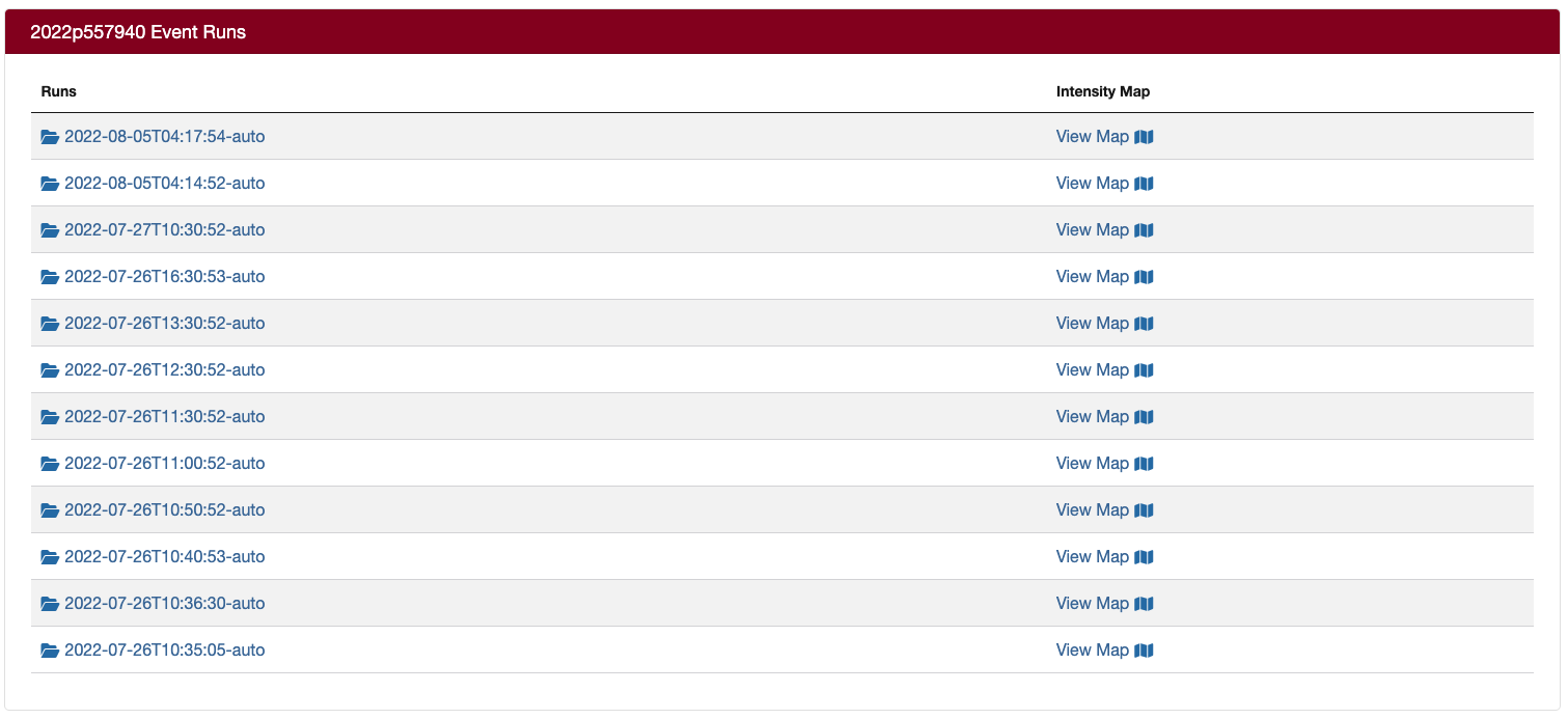
Each model run of the Shaking Layers tool is available in the 'Event Runs' page. Each 'Event Run' is a different version. A new run is due to a change in the input data. This could include the earthquake magnitude, location, ground motion observations, rupture characteristics or scientific configurations.
Each run is named with the date-time stamp (UTC time) when the run started (e.g. 2022-07-27T10:32:52), which in this example is 10:32:52am on the 27th of July 2022. The run name also includes the type of run, which could be auto, reviewed, or revised.
Auto: Automatic runs are generated automatically by the Shaking Layers computer system. They use basic earthquake parameters and recorded strong motion data as inputs. Automatic runs have not been reviewed by a human. Automatic runs are triggered when a earthquake solution (magnitude, location, depth) changes, or at certain time intervals after and earthquake when new strong motion data may be available.
Reviewed: A reviewed run has been reviewed by a seismologist and updated based on any available science before publishing. A reviewed run may include new scientific input data such as an earthquake fault rupture geometry, felt reports, additional strong motion data, earthquake tectonic type information, and other configurations.
Revised: A revised run is an automatic run that has updated a previously reviewed run. This may include new strong motion data or changes to earthquake solutions.
The first runs of an Earthquake are always automatic and the first run can be expected approximately 20 minutes following an earthquake. Automatic runs occur frequently immediately after an earthquake due to changes in the earthquake solution which trigger an automatic run. Reviewed runs will generally only be available after significant earthquakes.
Input data
Input data for each run can be found in the raw file directory. This includes the earthquake source information (event.xml) and recorded strong motion data (event_dat.xml). Configuration details of the ShakeMap software (e.g. see model.conf and info.json) are also provided.
Updates
Shaking Layers technical configurations
Current default configurations
These configurations are applied to all automatically generated Shaking Layers. Some parameters (e.g. E and F) may be updated by GNS Seismologists with event-specific information in 'reviewed' versions of Shaking Layers.
| Configuration | Model | Current model | Start date | Comments | ShakeMap atlas |
|---|---|---|---|---|---|
| A | Vs30 (time-averaged shear-wave velocity in the uppermost 30 m of the subsurface) | Updated Foster et al model (unpublished, but available on https://github.com/ucgmsim/Vs30) | 8 March 2024 | All events from the ShakeMap atlas (1848-2020) use this model too | |
| B | GMPE Ground Motion Prediction Equation | Gerstenberger et al. (2024); Bradley et al. (2024) | March 2021 | The logic tree used in the 2022 update of the National Seismic Hazard Model (NSHM) | All events from the ShakeMap atlas (1848-2020) use this model too |
| C | GMICE Ground Motion to Intensity Conversion equation | Moratalla et al. (2021) | March 2021 | All events from the ShakeMap atlas (1848-2020) use this model too | |
| D | IPE Intensity Prediction equation | Allen et al. (2012) | March 2021 | All events from the ShakeMap atlas (1848-2020) use this model too | |
| E | Earthquake magnitude equation | Christophersen et al. (2022) | March 2021 | ||
| F | Default tectonic type assignment | Horspool et al. (2023) | March 2021 | This is for the initial shaking layers, when tectonic type is not known. Once identified, a deterministic tectonic type is being used in manually reviewed runs for the same event | All events from the ShakeMap atlas (1848-2020) use a deterministic tectonic type assignment based on the scientific information about that earthquake |
Past configurations
Previous versions of the above default configurations are shown below. Only models that have changed from the current models are shown in this table.
| Reference | Model | Past model | Start date | End date | Comments | ShakeMap atlas |
|---|---|---|---|---|---|---|
| A | Vs30 (time-averaged shear-wave velocity in the uppermost 30 m of the subsurface) | Perrin et al (2015) | March 2021 | 7 March 2024 | All events from the ShakeMap atlas (1848-2020) use this model too | |
| B | GMPE Ground Motion Prediction Equation | N/A | ||||
| C | GMICE Ground Motion to Intensity Conversion equation | N/A | ||||
| D | IPE Intensity Prediction equation | N/A | ||||
| E | Earthquake magnitude equation | N/A | ||||
| F | Default tectonic type assignment | N/A |
For further information, please refer to the guidelines:
Horspool NA, Kaiser AE, Goded T, Charlton DH, Moratalla JM, Chadwick MP, Groom J, Houltham J, Abbott ER, Andrews JR, et al. 2023. GNS Shaking Layers Tool: guidelines for end users. Lower Hutt (NZ): GNS Science. 64 p. (GNS Science report; 2023/13). https://doi.org/10.21420/VZKK-TP35
References
Allen TI, Wald DJ, Worden CB. 2012. Intensity attenuation for active crustal regions. Journal of Seismology. 16(3):409–433.https://doi.org/10.1007/s10950-012-9278-7
Bradley, B.A., S.S. Bora, R.L. Lee, E.F. Manea, M.C. Gerstenberger, P.J. Stafford, G.M. Atkinson, G. Weatherill, J. Hutchinson, C.A. de la Torre, A.M. Hulsey and A.E. Kaiser (2024). The ground-motion characterization model for the 2022 New Zealand National Seismic Hazard Model, Bull. Seismol. Soc. Am, 114(1): 329-349; doi: 10.1785/0120230170
Christophersen A, Bourguignon S, Rhoades DA, Allen TI, Salichon J, Ristau J, Rollins C, Gerstenberger MC. 2022. Consistent magnitudes over time for the revision of the New Zealand National Seismic Hazard Model. Lower Hutt (NZ): GNS Science. 76 p. (GNS Science report; 2021/42). https://doi.org/10.21420/A2SN-XM76
Gerstenberger, M.C., S.S. Bora, B.A. Bradley, C. DiCaprio, A.E. Kaiser, E.F. Manea, A. Nicol, J.C. Rollins, M.W. Stirling, K.K.S. Thingbaijam, R.J. Van Dissen, E.R. Abbott, G.M. Atkinson, C. Chamberlain, A. Christophersen, K.J. Clark, G.L. Coffey, C.A. de la Torre, S.M. Ellis, J. Fraser, K. Graham, J. Griffin, I.J. Hamling, M.P. Hill, A. Howell, A. Hulsey, J. Hutchinson, P. Iturrieta, K.M. Johnson, V.O. Jurgens, R. Kirkman, R.M. Langridge, R.L. Lee, N.J. Litchfield, J. Maurer, K.R. Milner, S.J. Rastin, M.S. Rattenbury, D.A. Rhoades, J. Ristau, D. Schorlemmer, H. Seebeck, B.E. Shaw, P.J. Stafford, A.C. Stolte, J. Townend, P. Villamor, L.M. Wallace, G. Weatherill, C.A. Williams and L.M. Wotherspoon (2023). The 2022 Aotearoa New Zealand National Seismic Hazard Model : process, overview, and results, Bull. Seismol. Soc. Am, 114(1):7-36; doi: 10.1785/0120230182
Horspool NA, Kaiser AE, Goded T, Charlton DH, Moratalla JM, Chadwick MP, Groom J, Houltham J, Abbott ER, Andrews JR, et al. 2023. GNS Shaking Layers Tool: guidelines for end users. Lower Hutt (NZ): GNS Science. 64 p. (GNS Science report; 2023/13). https://doi.org/10.21420/VZKK-TP35
Moratalla JM, Goded T, Rhoades DA, Canessa S, Gerstenberger MC. 2021. New ground motion to intensity conversion equations (GMICEs) for New Zealand. Seismological Research Letters. 92(1):448–459. https://doi.org/10.1785/0220200156
Perrin ND, Heron DW, Kaiser AE, Van Houtte C. 2015. VS30 and NZS 1170.5 site class maps of New Zealand. In: New dimensions in earthquake resilience: 2015 New Zealand Society for Earthquake Engineering Technical Conference and AGM; 2015 Apr 10–12; Rotorua, New Zealand. Wellington (NZ): New Zealand Society for Earthquake Engineering. Paper O-07.
Earthquake Magnitude
The initial magnitude from GeoNet is used as automated input into ShakeMap. GeoNet provides a summary magnitude (M) that is influenced by local magnitude (ML), whereas ShakeMap requires a moment magnitude (MW). To convert between local and moment magnitude for the automatic map generation, the following equation is applied, based on the average correction value between these two metrics derived by Christophersen et al. (2022, pers. comm.):
Equation
The Shaking Layers magnitude may be updated by GNS Science seismologists in reviewed versions of shaking layers. For very large earthquakes, a MWW derived from w-phase inversion (Duputel et al. 2012) is considered the global international standard because it provides robust magnitudes that do not saturate (i.e. are not under-estimated in the largest earthquakes). W‑phase inversions for New Zealand are now generated by the R-CET programme within 18–30 minutes of large earthquakes in New Zealand and the southwest Pacific (subject to quality criteria being met) (Fry et al. 2022). W-phase solutions are also available on variable timeframes from international agencies USGS or Geoscience Australia. For small to moderate earthquakes, MW may also be directly estimated from Regional Moment Tensor inversion (e.g. Ristau 2013).
These configurations may change in the future. Please check for any updates at https://shakinglayers.geonet.org.nz/html/guidelines#updates
File types
Standard files
The standard file set are a set of files produced from the raw files that are stable and supported by GeoNet. The standard files are available through the Shaking Layers API. The standard files are very unlikely to change and if there are changes, GeoNet users will be notified.
Standard file type descriptions
| File Name | File Format | Intensity Measure Type | Intensity Measure Type Unit |
Description |
|---|---|---|---|---|
| intensity_mmi.tif | Geotiff | Intensity | MMI | Raster grid of intensity |
| intensity_mmi_stddev.tif | Geotiff | Intensity | MMI | Raster grid of intensity standard deviation (uncertainty) |
| intensity_mmi_contour_lines.json | Geojson | Intensity | MMI | Generalised contour lines of intensity |
| intensity_mmi_contour_polygons.zip | Shapefile (in a zipped file) | Intensity | MMI | Detailed contoured polygons of intensity |
| intensity_mmi_map.pdf | Intensity | MMI | Static map of intensity with strong motion stations | |
| pga_g.tif | Geotiff | Peak ground acceleration (PGA) | g | Raster grid of PGA |
| pga_g_stddev.tif | Geotiff | Peak ground acceleration (PGA) | log(g) | Raster grid of PGA standard deviation (uncertainty) |
| pga_g_contour_lines.json | Geojson | Peak ground acceleration (PGA) | g | Generalised contour lines of PGA |
| pga_g_contour_polygons.zip | Shapefile (in a zipped file) | Peak ground acceleration (PGA) | g | Detailed contoured polygons of PGA |
| pgv_cms.tif | Geotiff | Peak ground velocity (PGV) | cm/s | Raster grid of PGV |
| pgv_cms_stddev.tif | Geotiff | Peak ground velocity (PGV) | cm/s | Raster grid of PGV standard deviation (uncertainty) |
| pgv_cms_contour_lines.json | Geojson | Peak ground velocity (PGV) | cm/s | Generalised contour lines of PGV |
| pgv_cms_contour_polygons.zip | Shapefile (in a zipped file) | Peak ground velocity (PGV) | cm/s | Detailed contoured polygons of PGV |
| psa_0p3_g.tif | Geotiff | Pseudo-spectral acceleration (PSA) for 0.3s period | g | Raster grid of PSA for 0.3s period |
| psa_0p3_g_stddev.tif | Geotiff | Pseudo-spectral acceleration (PSA) for 0.3s period | log(g) | Raster grid of PSA for 0.3s period standard deviation (uncertainty) |
| psa_0p3_g_contour_lines.json | Geojson | Pseudo-spectral acceleration (PSA) for 0.3s period | g | Generalised contour lines of PSA for 0.3s period |
| psa_0p3_g_contour_polygons.zip | Shapefile (in a zipped file) | Pseudo-spectral acceleration (PSA) for 0.3s period | g | Detailed contoured polygons of PSA for 0.3s period |
| psa_1p0_g.tif | Geotiff | Pseudo-spectral acceleration (PSA) for 1.0s period | g | Raster grid of PSA for 1.0s period |
| psa_1p0_g_stddev.tif | Geotiff | Pseudo-spectral acceleration (PSA) for 1.0s period | log(g) | Raster grid of PSA for 1.0s period standard deviation (uncertainty) |
| psa_1p0_g_contour_lines.json | Geojson | Pseudo-spectral acceleration (PSA) for 1.0s period | g | Generalised contour lines of PSA for 1.0s period |
| psa_1p0_g_contour_polygons.zip | Shapefile (in a zipped file) | Pseudo-spectral acceleration (PSA) for 1.0s period | g | Detailed contoured polygons of PSA for 1.0s period |
| psa_3p0_g.tif | Geotiff | Pseudo-spectral acceleration (PSA) for 3.0s period | g | Raster grid of PSA for 3.0s period |
| psa_3p0_g_stddev.tif | Geotiff | Pseudo-spectral acceleration (PSA) for 3.0s period | log(g) | Raster grid of PSA for 3.0s period standard deviation (uncertainty) |
| psa_3p0_g_contour_lines.json | Geojson | Pseudo-spectral acceleration (PSA) for 3.0s period | g | Generalised contour lines of PSA for 3.0s period |
| psa_3p0_g_contour_polygons.zip | Shapefile (in a zipped file) | Pseudo-spectral acceleration (PSA) for 3.0s period | g | Detailed contoured polygons of PSA for 3.0s period |
| param.json | Json | - | - | Dictionary of earthquake and model parameters |
Raw files
The raw file set consists of default files that are generated by the ShakeMap software used to create Shaking Layers information. The raw files are not supported by GeoNet and may change at any time without warning.
For information on the raw files please refer to the USGS ShakeMap website.
Using Shaking Layers
Software compatibility
Geotiff: Geotiff is a raster file that can be opened in a Geographic Information System (GIS) software such as QGIS (free and open source) or ArcGIS (license required).
Shapefile: Shapefiles are a vector file.
GeoJson: Geojson is an open data format for representing vector geographic features. Geojson can be opened in GIS software or in the geojson website.
Json: Json is a human and computer readable format. Json files can be viewed in a text editor or a web browser.
PDF: PDF files should open in the Web Browser when clicked. PDF files that are downloaded can be viewed in a PDF viewer such as Adobe Acrobat Reader.
Coordinate system projection
All standard and raw files are projected in WGS84 (CRS 4326) which has units of decimal degrees.
Maps with uncertainty
The Shaking Layers tool produces the mean estimate of shaking (e.g. pga_g.tiff) as well as an estimate of the uncertainty (pga_g_std.tiff), represented by the standard deviation. Some users may be interested in producing a custom shaking map that combines these two layers. This can be undertaken in a raster calculator in a GIS system such as QGIS or ArcGIS or through a programming language such as Python or GDAL. Below we show the equation to combine the mean and standard deviation layers to produce a custom map.
In this example we want to calculate a conservative shaking map that shows the mean plus two standard deviation (i.e. the 95th percentile shaking). To do this the following equation would be used in a raster calculator:
mean_plus_2stddev.tiff = exp( log(pga_g.tiff) + (2 x pga_g_std.tiff))
First we convert the mean PGA layer (pga_g.tiff) into log space, as this is the units of the standard deviation file. We then multiply the standard deviation PGA layer (pga_g_std.tiff) by the number of standard deviations away from the mean. If we were interested in plus one standard deviation this number would be 1 instead of 2. We then add together both these numbers. If we were interested in the mean minus two standard deviations then we would subtract instead of adding. We then take the exponential of this value to convert out of log space.
How to cite
If you use Shaking Layers data, please use this citation:
GNS Science, GeoNet Shaking Layers Dataset. https://doi.org/10.21420/J856-2J84